require(gtsummary, quietly = TRUE, warn.conflicts = FALSE)
require(survival, quietly = TRUE, warn.conflicts = FALSE)
require(popEpi, quietly = TRUE, warn.conflicts = FALSE)
require(dplyr, quietly = TRUE, warn.conflicts = FALSE)
require(tidyr, quietly = TRUE, warn.conflicts = FALSE)
require(ggplot2, quietly = TRUE, warn.conflicts = FALSE)SpyCATS primary results manuscript analysis
Introduction
This file contains the analysis conducted for the SpyCATS study primary results manuscript (Armitage et al., 2023). Data frames used were cleaned and set up separately. Data used here only include necessary variables for the analysis included in this article. Requests for collaboration and access to additional study data can be made to Edwin.Armitage@lshtm.ac.uk.
Load necessary packages
Study recruitment numbers
The enrolment_visits dataframe contains the date and visit of the first (enrolment) visit of each participant.
load("./Data/enrolment_visits.RData")

head(enrolment_visits)
# A tibble: 6 × 5
pid hid date visit present
<chr> <chr> <date> <chr> <dbl>
1 00201K 002 2021-08-02 mv0 1
2 00202E 002 2021-09-14 mv1 1
3 00203F 002 2021-08-02 mv0 1
4 00204D 002 2021-08-02 mv0 1
5 00205G 002 2021-08-02 mv0 1
6 00206C 002 2022-05-17 mv9 1Total number of participants recruited.
enrolment_visits |>
  nrow()
[1] 442Total number of households recruited.
enrolment_visits |>
  distinct(hid) |>
  nrow()
[1] 44Participants recruited at MV0 and dates.
enrolment_visits |>
  filter(visit == "mv0") |>
  summarise(recruited_mv0 = n(), start_date = min(date), end_date = max(date))
# A tibble: 1 × 3
recruited_mv0 start_date end_date
<int> <date> <date>
1 337 2021-07-27 2021-09-02Participants recruited after MV0 and dates.
enrolment_visits |>
  filter(visit != "mv0") |>
  summarise(recruited_after_mv0 = n())
# A tibble: 1 × 1
recruited_after_mv0
<int>
1 105The final_visits dataframe contains the dates of all mv12 visits completed.
load("./Data/final_visits.RData")

final_visits |>
  summarise(completed_mv12 = n(), start_date = min(date), end_date = max(date))
# A tibble: 1 × 3
completed_mv12 start_date end_date
<int> <date> <date>
1 302 2022-06-28 2022-09-28Demographics
The demographics dataframe contains basic demographic information for each participant. N.B. Demogrphic data were not collected for one participant.
Demographic data for participants are included in TableS2.
load("./Data/demographics.RData")

head(demographics)
# A tibble: 6 × 6
# Rowwise:
pid age age_grp ethnicity sex median_hhsize
<chr> <int> <fct> <fct> <fct> <dbl>
1 00201K 33 Over 18 years Mandinka Male 6
2 00203F 21 Over 18 years Fula Female 6
3 00204D 3 0-4 years Fula Male 6
4 00205G 1 0-4 years Fula Male 6
5 00601F 27 Over 18 years Serehule Male 11
6 00602J 35 Over 18 years Serehule Male 11demographics |>
select(!pid & !median_hhsize) |>
tbl_summary(
label = list(age ~ "Median Age",
age_grp ~ "Age Group",
ethnicity ~ "Ethnicity",
sex ~ "Sex"),
statistic = list(all_continuous() ~ "{median} (IQR: {p25}-{p75}, range: {min}-{max})"),
missing_text = "(Missing)")| Characteristic | N = 4411 |
|---|---|
| Median Age | 15 (IQR: 6-28, range: 0-85) |
| Age Group | |
| 0-4 years | 104 (24%) |
| 5-11 years | 79 (18%) |
| 12-17 years | 73 (17%) |
| Over 18 years | 185 (42%) |
| Ethnicity | |
| Mandinka | 311 (71%) |
| Wolof | 30 (6.9%) |
| Fula | 43 (9.9%) |
| Jola | 17 (3.9%) |
| Serehule | 12 (2.8%) |
| Serere | 12 (2.8%) |
| Manjago | 6 (1.4%) |
| Non-African | 3 (0.7%) |
| Other | 2 (0.5%) |
| (Missing) | 5 |
| Sex | |
| Male | 208 (47%) |
| Female | 233 (53%) |
| 1 Median (IQR: 25%-75%, range: Minimum-Maximum); n (%) | |
Median household size calculated over number of households, not participants.
demographics |>
  mutate(hid = substr(pid,1,3)) |>
  distinct(hid, .keep_all = TRUE) |>
  select(median_hhsize) |>
  tbl_summary(
    label = list(median_hhsize ~ "Median Household Size"),
statistic = list(all_continuous() ~ "{median} (IQR: {p25}-{p75}, range: {min}-{max})"))| Characteristic | N = 441 |
|---|---|
| Median Household Size | 7.0 (IQR: 6.0-10.0, range: 4.0-37.0) |
| 1 Median (IQR: 25%-75%, range: Minimum-Maximum) | |
Follow up time
Follow up time was calculated separately for carriage and infection, as carriage events could only occur at monthly visits, so unscheduled follow up visits were not included in carriage follow up time. The infection_long and carriage_long dataframes contain entry and exit points in days from enrolment for each participant, with gap indicating whether the period is a gap in follow up.
Infection follow up time.
load("./Data/infection_long.RData")

head(infection_long)
pid tstart tstop gap
1 00201K 0.0 57.0 0
2 00201K 57.0 199.5 1
3 00201K 199.5 231.0 0
4 00203F 0.0 303.0 0
5 00204D 0.0 303.0 0
6 00205G 0.0 270.0 0# Gaps in follow up time are where gap == 1, so these are filtered out.
infection_long |>
filter(gap == 0) |>
mutate(time = tstop - tstart) |>
summarise(follow_up_time = sum(time)/365.25) follow_up_time
1 311.4148Carriage follow up time.
load("./Data/carriage_long.RData")

head(carriage_long)
pid tstart tstop gap
1 00201K 0.0 57.0 0
2 00201K 57.0 199.5 1
3 00201K 199.5 231.0 0
4 00203F 0.0 303.0 0
5 00204D 0.0 303.0 0
6 00205G 0.0 270.0 0# Gaps in follow up time are where gap == 1, so these are filtered out.
carriage_long |>
filter(gap == 0) |>
mutate(time = tstop - tstart) |>
summarise(follow_up_time = sum(time)/365.25) follow_up_time
1 307.5133Carriage and infection events
Carriage and infection events are defined according to criteria described in the manuscript. The events dataframe is a long dataset containing a row for each visit, so multiple rows per participant. Each of the variables gas_infection, gas_carriage, gas_pharyngitis, gas_pyoderma, gas_throat_carriage and gas_skin_carriage are 1 or 0 depending on whether the criteria for an event were met for that participant at that visit. pharyngitis and pyoderma are 1 or 0 depending on whether the participant was suffering from throat or skin symptoms at that visit.
load("./Data/events.RData")

glimpse(events)
Rows: 4,547
Columns: 11
$ pid <chr> "00201K", "00201K", "00201K", "00203F", "00203F", …
$ visit <chr> "mv0", "mv1", "mv7", "mv0", "mv1", "mv2", "mv3", "…
$ date <dbl> 0, 43, 210, 0, 43, 71, 93, 120, 161, 189, 210, 252…
$ pharyngitis <dbl> 0, 0, 0, 1, 0, 0, 0, 0, 0, 0, 0, 0, 0, 0, 0, 0, 0,…
$ pyoderma <dbl> 1, 0, 0, 0, 0, 0, 0, 0, 0, 0, 0, 0, 0, 1, 0, 0, 0,…
$ gas_pyoderma <dbl> 0, 0, 0, 0, 0, 0, 0, 0, 0, 0, 0, 0, 0, 0, 0, 0, 0,…
$ gas_pharyngitis <dbl> 0, 0, 0, 0, 0, 0, 0, 0, 0, 0, 0, 0, 0, 0, 0, 0, 0,…
$ gas_infection <dbl> 0, 0, 0, 0, 0, 0, 0, 0, 0, 0, 0, 0, 0, 0, 0, 0, 0,…
$ gas_throat_carriage <dbl> 0, 0, 0, 0, 0, 0, 0, 0, 0, 0, 0, 0, 0, 0, 0, 0, 0,…
$ gas_skin_carriage <dbl> 0, 0, 0, 0, 0, 0, 0, 0, 0, 0, 0, 0, 0, 0, 0, 0, 0,…
$ gas_carriage <dbl> 0, 0, 0, 0, 0, 0, 0, 0, 0, 0, 0, 0, 0, 0, 0, 0, 0,…Total events by event type.
events |>
  summarise(StrepA_pharyngitis = sum(gas_pharyngitis),
            StrepA_pyoderma = sum(gas_pyoderma),
            StrepA_throat_carriage = sum(gas_throat_carriage),
            StrepA_skin_carriage = sum(gas_skin_carriage))
# A tibble: 1 × 4
StrepA_pharyngitis StrepA_pyoderma StrepA_throat_carriage StrepA_skin_carriage
<dbl> <dbl> <dbl> <dbl>
1 17 99 49 39Checking for simultaneous events.
events |>
  tbl_cross(
    row = gas_pharyngitis,
col = gas_pyoderma)| gas_pyoderma | Total | ||
|---|---|---|---|
| 0 | 1 | ||
| gas_pharyngitis | |||
| 0 | 4,432 | 98 | 4,530 |
| 1 | 16 | 1 | 17 |
| Total | 4,448 | 99 | 4,547 |
events |>
  tbl_cross(
    row = gas_pharyngitis,
col = gas_skin_carriage)| gas_skin_carriage | Total | ||
|---|---|---|---|
| 0 | 1 | ||
| gas_pharyngitis | |||
| 0 | 4,491 | 39 | 4,530 |
| 1 | 17 | 0 | 17 |
| Total | 4,508 | 39 | 4,547 |
events |>
  tbl_cross(
    row = gas_pyoderma,
col = gas_throat_carriage)| gas_throat_carriage | Total | ||
|---|---|---|---|
| 0 | 1 | ||
| gas_pyoderma | |||
| 0 | 4,402 | 46 | 4,448 |
| 1 | 96 | 3 | 99 |
| Total | 4,498 | 49 | 4,547 |
events |>
  tbl_cross(
    row = gas_pyoderma,
col = gas_skin_carriage)| gas_skin_carriage | Total | ||
|---|---|---|---|
| 0 | 1 | ||
| gas_pyoderma | |||
| 0 | 4,413 | 35 | 4,448 |
| 1 | 95 | 4 | 99 |
| Total | 4,508 | 39 | 4,547 |
Baseline carriage and infection prevalence
Baseline events are defined as carriage or infection that was present at a participant’s enrolment visit, whether they enrolled at MV0 or a later MV. The baseline dataframe contains each participant’s enrolment visit along with variables indicating whether they had infection or carriage at that visit.
load("./Data/baseline.RData")

head(baseline)
# A tibble: 6 × 8
pid visit gas_pharyngitis gas_pyoderma gas_throat_carriage gas_skin_carriage
<chr> <chr> <dbl> <dbl> <dbl> <dbl>
1 0020… mv0 0 0 0 0
2 0020… mv1 0 0 0 0
3 0020… mv0 0 0 0 0
4 0020… mv0 0 0 0 0
5 0020… mv0 0 0 0 0
6 0020… mv9 0 0 0 0
# ℹ 2 more variables: sex <fct>, age_grp <fct>Baseline prevalence of carriage and infection.
baseline |>
  select(contains("gas")) |>
  tbl_summary(label = list(gas_pharyngitis ~ "StrepA pharyngitis",
                           gas_throat_carriage ~ "StrepA pharyngeal carriage",
                           gas_pyoderma ~ "StrepA pyoderma",
                           gas_skin_carriage ~ "StrepA skin carriage")) |>
add_ci(method = list(everything() ~ "exact"))| Characteristic | N = 4421 | 95% CI2 |
|---|---|---|
| StrepA pharyngitis | 1 (0.2%) | 0.01%, 1.3% |
| StrepA pyoderma | 17 (3.8%) | 2.3%, 6.1% |
| StrepA pharyngeal carriage | 12 (2.7%) | 1.4%, 4.7% |
| StrepA skin carriage | 1 (0.2%) | 0.01%, 1.3% |
| 1 n (%) | ||
| 2 CI = Confidence Interval | ||
Baseline carriage and infection by sex.
baseline |>
  select(sex, contains("gas")) |>
  tbl_summary(
    label = list(gas_pharyngitis ~ "StrepA pharyngitis",
                           gas_throat_carriage ~ "StrepA pharyngeal carriage",
                           gas_pyoderma ~ "StrepA pyoderma",
                           gas_skin_carriage ~ "StrepA skin carriage"),
    by = sex,
    percent = "column") |>
  add_ci(method = list(everything() ~ "exact"))
1 observations missing `sex` have been removed. To include these observations, use `forcats::fct_na_value_to_level()` on `sex` column before passing to `tbl_summary()`.| Characteristic | Male, N = 2081 | 95% CI2 | Female, N = 2331 | 95% CI2 |
|---|---|---|---|---|
| StrepA pharyngitis | 0 (0%) | 0.00%, 1.8% | 1 (0.4%) | 0.01%, 2.4% |
| StrepA pyoderma | 11 (5.3%) | 2.7%, 9.3% | 6 (2.6%) | 0.95%, 5.5% |
| StrepA pharyngeal carriage | 6 (2.9%) | 1.1%, 6.2% | 6 (2.6%) | 0.95%, 5.5% |
| StrepA skin carriage | 1 (0.5%) | 0.01%, 2.6% | 0 (0%) | 0.00%, 1.6% |
| 1 n (%) | ||||
| 2 CI = Confidence Interval | ||||
Baseline carriage and infection by age group.
baseline |>
  select(age_grp, contains("gas")) |>
  tbl_summary(
    label = list(gas_pharyngitis ~ "StrepA pharyngitis",
                           gas_throat_carriage ~ "StrepA pharyngeal carriage",
                           gas_pyoderma ~ "StrepA pyoderma",
                           gas_skin_carriage ~ "StrepA skin carriage"),
    by = age_grp,
    percent = "column") |>
  add_ci(method = list(everything() ~ "exact"))
1 observations missing `age_grp` have been removed. To include these observations, use `forcats::fct_na_value_to_level()` on `age_grp` column before passing to `tbl_summary()`.| Characteristic | 0-4 years, N = 1041 | 95% CI2 | 5-11 years, N = 791 | 95% CI2 | 12-17 years, N = 731 | 95% CI2 | Over 18 years, N = 1851 | 95% CI2 |
|---|---|---|---|---|---|---|---|---|
| StrepA pharyngitis | 1 (1.0%) | 0.02%, 5.2% | 0 (0%) | 0.00%, 4.6% | 0 (0%) | 0.00%, 4.9% | 0 (0%) | 0.00%, 2.0% |
| StrepA pyoderma | 6 (5.8%) | 2.1%, 12% | 3 (3.8%) | 0.79%, 11% | 7 (9.6%) | 3.9%, 19% | 1 (0.5%) | 0.01%, 3.0% |
| StrepA pharyngeal carriage | 2 (1.9%) | 0.23%, 6.8% | 4 (5.1%) | 1.4%, 12% | 3 (4.1%) | 0.86%, 12% | 3 (1.6%) | 0.34%, 4.7% |
| StrepA skin carriage | 0 (0%) | 0.00%, 3.5% | 1 (1.3%) | 0.03%, 6.9% | 0 (0%) | 0.00%, 4.9% | 0 (0%) | 0.00%, 2.0% |
| 1 n (%) | ||||||||
| 2 CI = Confidence Interval | ||||||||
Monthly carriage prevalence
Monthly carriage prevalence was defined as the proportion of those swabbed at each monthly visit with carriage. In the monthly_carriage dataframe, for each participant there is a variable for each monthly visit indicating whether they were positive (1) or negative (0) for throat carriage or skin carriage, or were absent (NA).
load("./Data/monthly_carriage.RData")

head(monthly_carriage)
# A tibble: 6 × 32
pid mv0_gas_throat_carriage mv1_gas_throat_carriage mv2_gas_throat_carriage
<chr> <dbl> <dbl> <dbl>
1 00201K 0 0 NA
2 00203F 0 0 0
3 00204D 0 0 0
4 00205G 0 0 0
5 00601F 0 NA 0
6 00602J 0 NA NA
# ℹ 28 more variables: mv3_gas_throat_carriage <dbl>,
# mv4_gas_throat_carriage <dbl>, mv5_gas_throat_carriage <dbl>,
# mv6_gas_throat_carriage <dbl>, mv7_gas_throat_carriage <dbl>,
# mv8_gas_throat_carriage <dbl>, mv9_gas_throat_carriage <dbl>,
# mv10_gas_throat_carriage <dbl>, mv11_gas_throat_carriage <dbl>,
# mv12_gas_throat_carriage <dbl>, mv0_gas_skin_carriage <dbl>,
# mv1_gas_skin_carriage <dbl>, mv2_gas_skin_carriage <dbl>, …Monthly pharyngeal carriage prevalence.
monthly_carriage |>
  select(contains("gas_throat")) |>
  tbl_summary(
    label = list(mv0_gas_throat_carriage ~ "MV0",
                 mv1_gas_throat_carriage ~ "MV1",
                 mv2_gas_throat_carriage ~ "MV2",
                 mv3_gas_throat_carriage ~ "MV3",
                 mv4_gas_throat_carriage ~ "MV4",
                 mv5_gas_throat_carriage ~ "MV5",
                 mv6_gas_throat_carriage ~ "MV6",
                 mv7_gas_throat_carriage ~ "MV7",
                 mv8_gas_throat_carriage ~ "MV8",
                 mv9_gas_throat_carriage ~ "MV9",
                 mv10_gas_throat_carriage ~ "MV10",
                 mv11_gas_throat_carriage ~ "MV11",
                 mv12_gas_throat_carriage ~ "MV12"),
    type = everything() ~ "categorical",
    missing_text = "(Missing)") |>
  add_ci(method = list(everything() ~ "exact")) |>
modify_caption("**Pharyngeal Carriage**")| Characteristic | N = 4421 | 95% CI2 |
|---|---|---|
| MV0 | ||
| 0 | 330 (98%) | 96%, 99% |
| 1 | 7 (2.1%) | 0.84%, 4.2% |
| (Missing) | 105 | |
| MV1 | ||
| 0 | 319 (98%) | 96%, 99% |
| 1 | 6 (1.8%) | 0.68%, 4.0% |
| (Missing) | 117 | |
| MV2 | ||
| 0 | 264 (99%) | 96%, 100% |
| 1 | 4 (1.5%) | 0.41%, 3.8% |
| (Missing) | 174 | |
| MV3 | ||
| 0 | 249 (98%) | 95%, 99% |
| 1 | 5 (2.0%) | 0.64%, 4.5% |
| (Missing) | 188 | |
| MV4 | ||
| 0 | 253 (97%) | 94%, 99% |
| 1 | 8 (3.1%) | 1.3%, 5.9% |
| (Missing) | 181 | |
| MV5 | ||
| 0 | 264 (98%) | 96%, 99% |
| 1 | 5 (1.9%) | 0.61%, 4.3% |
| (Missing) | 173 | |
| MV6 | ||
| 0 | 263 (98%) | 95%, 99% |
| 1 | 6 (2.2%) | 0.82%, 4.8% |
| (Missing) | 173 | |
| MV7 | ||
| 0 | 248 (100%) | 98%, 100% |
| 1 | 1 (0.4%) | 0.01%, 2.2% |
| (Missing) | 193 | |
| MV8 | ||
| 0 | 246 (99%) | 97%, 100% |
| 1 | 2 (0.8%) | 0.10%, 2.9% |
| (Missing) | 194 | |
| MV9 | ||
| 0 | 245 (99%) | 97%, 100% |
| 1 | 2 (0.8%) | 0.10%, 2.9% |
| (Missing) | 195 | |
| MV10 | ||
| 0 | 246 (99%) | 97%, 100% |
| 1 | 2 (0.8%) | 0.10%, 2.9% |
| (Missing) | 194 | |
| MV11 | ||
| 0 | 247 (100%) | 98%, 100% |
| 1 | 1 (0.4%) | 0.01%, 2.2% |
| (Missing) | 194 | |
| MV12 | ||
| 0 | 300 (99%) | 98%, 100% |
| 1 | 2 (0.7%) | 0.08%, 2.4% |
| (Missing) | 140 | |
| 1 n (%) | ||
| 2 CI = Confidence Interval | ||
Monthly skin carriage prevalence.
monthly_carriage |>
  select(contains("gas_skin")) |>
  tbl_summary(
    label = list(mv0_gas_skin_carriage ~ "MV0",
                 mv1_gas_skin_carriage ~ "MV1",
                 mv2_gas_skin_carriage ~ "MV2",
                 mv3_gas_skin_carriage ~ "MV3",
                 mv4_gas_skin_carriage ~ "MV4",
                 mv5_gas_skin_carriage ~ "MV5",
                 mv6_gas_skin_carriage ~ "MV6",
                 mv7_gas_skin_carriage ~ "MV7",
                 mv8_gas_skin_carriage ~ "MV8",
                 mv9_gas_skin_carriage ~ "MV9",
                 mv10_gas_skin_carriage ~ "MV10",
                 mv11_gas_skin_carriage ~ "MV11",
                 mv12_gas_skin_carriage ~ "MV12"),
    type = everything() ~ "categorical",
    missing_text = "(Missing)") |>
  add_ci(method = list(everything() ~ "exact")) |>
modify_caption("**Skin Carriage**")| Characteristic | N = 4421 | 95% CI2 |
|---|---|---|
| MV0 | ||
| 0 | 336 (100%) | 98%, 100% |
| 1 | 1 (0.3%) | 0.01%, 1.6% |
| (Missing) | 105 | |
| MV1 | ||
| 0 | 324 (100%) | 98%, 100% |
| 1 | 1 (0.3%) | 0.01%, 1.7% |
| (Missing) | 117 | |
| MV2 | ||
| 0 | 264 (99%) | 96%, 100% |
| 1 | 4 (1.5%) | 0.41%, 3.8% |
| (Missing) | 174 | |
| MV3 | ||
| 0 | 252 (99%) | 97%, 100% |
| 1 | 2 (0.8%) | 0.10%, 2.8% |
| (Missing) | 188 | |
| MV4 | ||
| 0 | 254 (97%) | 95%, 99% |
| 1 | 7 (2.7%) | 1.1%, 5.4% |
| (Missing) | 181 | |
| MV5 | ||
| 0 | 263 (98%) | 95%, 99% |
| 1 | 6 (2.2%) | 0.82%, 4.8% |
| (Missing) | 173 | |
| MV6 | ||
| 0 | 267 (99%) | 97%, 100% |
| 1 | 2 (0.7%) | 0.09%, 2.7% |
| (Missing) | 173 | |
| MV7 | ||
| 0 | 249 (100%) | 99%, 100% |
| (Missing) | 193 | |
| MV8 | ||
| 0 | 244 (98%) | 96%, 100% |
| 1 | 4 (1.6%) | 0.44%, 4.1% |
| (Missing) | 194 | |
| MV9 | ||
| 0 | 243 (98%) | 96%, 100% |
| 1 | 4 (1.6%) | 0.44%, 4.1% |
| (Missing) | 195 | |
| MV10 | ||
| 0 | 248 (100%) | 99%, 100% |
| (Missing) | 194 | |
| MV11 | ||
| 0 | 241 (97%) | 94%, 99% |
| 1 | 7 (2.8%) | 1.1%, 5.7% |
| (Missing) | 194 | |
| MV12 | ||
| 0 | 299 (99%) | 97%, 100% |
| 1 | 3 (1.0%) | 0.21%, 2.9% |
| (Missing) | 140 | |
| 1 n (%) | ||
| 2 CI = Confidence Interval | ||
Mean monthly prevalence.
monthly_carriage |>
  pivot_longer(contains("gas"), names_to = c("visit",".value"), names_pattern = "([^_]*)_(.*)") |>
  group_by(visit) |>
  summarise(
    throat_carriage = mean(gas_throat_carriage, na.rm = TRUE),
    skin_carriage = mean(gas_skin_carriage, na.rm = TRUE),
    n_throat = sum(!is.na(gas_throat_carriage)),
    n_skin = sum(!is.na(gas_skin_carriage))) |>
  summarise(
    throat_carriage_mean = mean(throat_carriage),
    skin_carriage_mean = mean(skin_carriage),
    n_throat_total = sum(n_throat),
    n_skin_total = sum(n_skin),
    ci_lower_throat = binom.test(round(throat_carriage_mean * n_throat_total),
                                 n_throat_total)$conf.int[1],
    ci_upper_throat = binom.test(round(throat_carriage_mean * n_throat_total),
                                 n_throat_total)$conf.int[2],
    ci_lower_skin = binom.test(round(skin_carriage_mean * n_skin_total),
                               n_skin_total)$conf.int[1],
    ci_upper_skin = binom.test(round(skin_carriage_mean * n_skin_total),
                               n_skin_total)$conf.int[2]) |>
  print(width = Inf)
# A tibble: 1 × 8
throat_carriage_mean skin_carriage_mean n_throat_total n_skin_total
<dbl> <dbl> <int> <int>
1 0.0142 0.0120 3525 3525
ci_lower_throat ci_upper_throat ci_lower_skin ci_upper_skin
<dbl> <dbl> <dbl> <dbl>
1 0.0105 0.0187 0.00860 0.0161Incidence
Incidence is calculated by using the tmerge function of the survival package to create long dataframes for each of the relevant events with a row for each timepoint for each participant. This is done separately for each event type to avoid errors. The rate function from popEpi is then used to calculate overall and stratified incidence rates per 1000 person years of follow up.
Any infection incidence.
# merge infection_long and events, keeping only the rows where gas_infection == 1
incidence_gas_infection <- tmerge(infection_long, events |> filter(gas_infection == 1),
                                  id=pid, gas_infection = event(date, gas_infection))

# join incidence_gas_infection with demographics
incidence_gas_infection <- left_join(incidence_gas_infection, demographics)
Joining with `by = join_by(pid)`# keep only rows where gap == 0, and create a new variable called pyrs, which is the number of years between tstart and tstop
incidence_gas_infection <- incidence_gas_infection |>
filter(gap == 0) |>
mutate(pyrs = (tstop - tstart) / 365.25)
head(incidence_gas_infection) pid tstart tstop gap gas_infection age age_grp ethnicity sex
1 00201K 0.0 57 0 0 33 Over 18 years Mandinka Male
2 00201K 199.5 231 0 0 33 Over 18 years Mandinka Male
3 00203F 0.0 303 0 0 21 Over 18 years Fula Female
4 00204D 0.0 175 0 1 3 0-4 years Fula Male
5 00204D 175.0 303 0 0 3 0-4 years Fula Male
6 00205G 0.0 175 0 1 1 0-4 years Fula Male
median_hhsize pyrs
1 6 0.1560575
2 6 0.0862423
3 6 0.8295688
4 6 0.4791239
5 6 0.3504449
6 6 0.4791239table1 <- rate(incidence_gas_infection, obs = gas_infection, pyrs = pyrs/1000)
table2 <- rate(incidence_gas_infection, obs = gas_infection, pyrs = pyrs/1000, print = sex)
table3 <- rate(incidence_gas_infection, obs = gas_infection, pyrs = pyrs/1000, print = age_grp)
round_fun <- function(table) {
table |>
mutate(
rate = round(as.numeric(rate)),
rate.lo = round(as.numeric(rate.lo)),
rate.hi = round(as.numeric(rate.hi)))
}
round_fun(table1)
Crude rates and 95% confidence intervals:

   gas_infection         / rate  SE.rate rate.lo rate.hi
1: 97 0.3114148 311 31.62617 255 380round_fun(table2)
Crude rates and 95% confidence intervals:

      sex gas_infection         / rate  SE.rate rate.lo rate.hi
1:   Male            70 0.1374914  509 60.85179     403     644
2: Female 27 0.1738809 155 29.88340 106 226round_fun(table3)
Crude rates and 95% confidence intervals:

         age_grp gas_infection          / rate  SE.rate rate.lo rate.hi
1:     0-4 years            48 0.08848118  542 78.30144     409     720
2:    5-11 years            30 0.05826215  515 94.01002     360     736
3:   12-17 years             8 0.04129021  194 68.50115      97     387
4: Over 18 years            11 0.12333881   89 26.89036      49     161
Pharyngitis incidence.
incidence_gas_pharyngitis <- tmerge(infection_long, events |> filter(gas_pharyngitis == 1),
                                  id=pid, gas_pharyngitis = event(date, pharyngitis))

incidence_gas_pharyngitis <- left_join(incidence_gas_pharyngitis, demographics)
Joining with `by = join_by(pid)`incidence_gas_pharyngitis <- incidence_gas_pharyngitis |>
filter(gap == 0) |>
mutate(pyrs = (tstop - tstart) / 365.25)
table1 <- rate(incidence_gas_pharyngitis, obs = gas_pharyngitis, pyrs = pyrs/1000)
table2 <- rate(incidence_gas_pharyngitis, obs = gas_pharyngitis, pyrs = pyrs/1000, print = sex)
table3 <- rate(incidence_gas_pharyngitis, obs = gas_pharyngitis, pyrs = pyrs/1000, print = age_grp)
round_fun(table1)
Crude rates and 95% confidence intervals:

   gas_pharyngitis         / rate  SE.rate rate.lo rate.hi
1: 16 0.3114148 51 12.84461 31 84round_fun(table2)
Crude rates and 95% confidence intervals:

      sex gas_pharyngitis         / rate  SE.rate rate.lo rate.hi
1:   Male               8 0.1374914   58 20.57166      29     116
2: Female 8 0.1738809 46 16.26646 23 92round_fun(table3)
Crude rates and 95% confidence intervals:

         age_grp gas_pharyngitis          / rate  SE.rate rate.lo rate.hi
1:     0-4 years               2 0.08848118   23 15.98321       6      90
2:    5-11 years               7 0.05826215  120 45.41115      57     252
3:   12-17 years               2 0.04129021   48 34.25058      12     194
4: Over 18 years               5 0.12333881   41 18.12948      17      97
gas_pharyngitis_cases <- pull(table1[1,1])Pyoderma incidence.
incidence_gas_pyoderma <- tmerge(infection_long, events |> filter(gas_pyoderma == 1),
                                  id=pid, gas_pyoderma = event(date, gas_pyoderma))

incidence_gas_pyoderma <- left_join(incidence_gas_pyoderma, demographics)
Joining with `by = join_by(pid)`incidence_gas_pyoderma <- incidence_gas_pyoderma |>
filter(gap == 0) |>
mutate(pyrs = (tstop - tstart) / 365.25)
table1 <- rate(incidence_gas_pyoderma, obs = gas_pyoderma, pyrs = pyrs/1000)
table2 <- rate(incidence_gas_pyoderma, obs = gas_pyoderma, pyrs = pyrs/1000, print = sex)
table3 <- rate(incidence_gas_pyoderma, obs = gas_pyoderma, pyrs = pyrs/1000, print = age_grp)
round_fun(table1)
Crude rates and 95% confidence intervals:

   gas_pyoderma         / rate  SE.rate rate.lo rate.hi
1: 82 0.3114148 263 29.07821 212 327round_fun(table2)
Crude rates and 95% confidence intervals:

      sex gas_pyoderma         / rate  SE.rate rate.lo rate.hi
1:   Male           63 0.1374914  458 57.72908     358     587
2: Female 19 0.1738809 109 25.06830 70 171round_fun(table3)
Crude rates and 95% confidence intervals:

         age_grp gas_pyoderma          / rate  SE.rate rate.lo rate.hi
1:     0-4 years           46 0.08848118  520 76.65280     389     694
2:    5-11 years           24 0.05826215  412 84.08511     276     615
3:   12-17 years            6 0.04129021  145 59.32374      65     323
4: Over 18 years            6 0.12333881   49 19.85985      22     108
gas_pyoderma_cases <- pull(table1[1,1])Carriage incidence is calculated in the same way but using the carriage_long dataframe.
Throat or skin carriage incidence.
incidence_gas_carriage <- tmerge(carriage_long, events |> filter(gas_carriage == 1), id=pid,
                                gas_carriage = event(date, gas_carriage))
incidence_gas_carriage <- left_join(incidence_gas_carriage, demographics)
Joining with `by = join_by(pid)`incidence_gas_carriage <- incidence_gas_carriage |>
filter(gap ==0) |>
mutate(pyrs = (tstop - tstart) / 365.25)
table1 <- rate(incidence_gas_carriage, obs = gas_carriage, pyrs = pyrs/1000)
table2 <- rate(incidence_gas_carriage, obs = gas_carriage, pyrs = pyrs/1000, print = sex)
table3 <- rate(incidence_gas_carriage, obs = gas_carriage, pyrs = pyrs/1000, print = age_grp)
round_fun(table1)
Crude rates and 95% confidence intervals:

   gas_carriage         / rate  SE.rate rate.lo rate.hi
1: 75 0.3075133 244 28.16221 194 306round_fun(table2)
Crude rates and 95% confidence intervals:

      sex gas_carriage         / rate  SE.rate rate.lo rate.hi
1:   Male           49 0.1355722  361 51.63300     273     478
2: Female 26 0.1718987 151 29.66293 103 222round_fun(table3)
Crude rates and 95% confidence intervals:

         age_grp gas_carriage          / rate  SE.rate rate.lo rate.hi
1:     0-4 years           36 0.08793634  409 68.23117     295     568
2:    5-11 years           24 0.05710404  420 85.79042     282     627
3:   12-17 years            8 0.04070294  197 69.48950      98     393
4: Over 18 years            7 0.12172758   58 21.73502      27     121
Throat carriage incidence.
incidence_gas_throat_carriage <- tmerge(carriage_long, events |> filter(gas_throat_carriage == 1), id=pid,
                                gas_throat_carriage = event(date, gas_throat_carriage))
incidence_gas_throat_carriage <- left_join(incidence_gas_throat_carriage, demographics)
Joining with `by = join_by(pid)`incidence_gas_throat_carriage <- incidence_gas_throat_carriage |>
filter(gap ==0) |>
mutate(pyrs = (tstop - tstart) / 365.25)
table1 <- rate(incidence_gas_throat_carriage, obs = gas_throat_carriage, pyrs = pyrs/1000)
table2 <- rate(incidence_gas_throat_carriage, obs = gas_throat_carriage, pyrs = pyrs/1000, print = sex)
table3 <- rate(incidence_gas_throat_carriage, obs = gas_throat_carriage, pyrs = pyrs/1000, print = age_grp)
round_fun(table1)
Crude rates and 95% confidence intervals:

   gas_throat_carriage         / rate  SE.rate rate.lo rate.hi
1: 37 0.3075133 120 19.78048 87 166round_fun(table2)
Crude rates and 95% confidence intervals:

      sex gas_throat_carriage         / rate  SE.rate rate.lo rate.hi
1:   Male                  22 0.1355722  162 34.59718     107     246
2: Female 15 0.1718987 87 22.53061 53 145round_fun(table3)
Crude rates and 95% confidence intervals:

         age_grp gas_throat_carriage          / rate  SE.rate rate.lo rate.hi
1:     0-4 years                  15 0.08793634  171 44.04303     103     283
2:    5-11 years                  14 0.05710404  245 65.52352     145     414
3:   12-17 years                   2 0.04070294   49 34.74475      12     196
4: Over 18 years                   6 0.12172758   49 20.12272      22     110
Skin carriage incidence.
incidence_gas_skin_carriage <- tmerge(carriage_long, events |> filter(gas_skin_carriage == 1), id=pid,
                                gas_skin_carriage = event(date, gas_skin_carriage))
incidence_gas_skin_carriage <- left_join(incidence_gas_skin_carriage, demographics)
Joining with `by = join_by(pid)`incidence_gas_skin_carriage <- incidence_gas_skin_carriage |>
filter(gap ==0) |>
mutate(pyrs = (tstop - tstart) / 365.25)
table1 <- rate(incidence_gas_skin_carriage, obs = gas_skin_carriage, pyrs = pyrs/1000)
table2 <- rate(incidence_gas_skin_carriage, obs = gas_skin_carriage, pyrs = pyrs/1000, print = sex)
table3 <- rate(incidence_gas_skin_carriage, obs = gas_skin_carriage, pyrs = pyrs/1000, print = age_grp)
round_fun(table1)
Crude rates and 95% confidence intervals:

   gas_skin_carriage         / rate SE.rate rate.lo rate.hi
1: 38 0.3075133 124 20.046 90 170round_fun(table2)
Crude rates and 95% confidence intervals:

      sex gas_skin_carriage         / rate  SE.rate rate.lo rate.hi
1:   Male                27 0.1355722  199 38.32756     137     290
2: Female 11 0.1718987 64 19.29407 35 116round_fun(table3)
Crude rates and 95% confidence intervals:

         age_grp gas_skin_carriage          / rate   SE.rate rate.lo rate.hi
1:     0-4 years                21 0.08793634  239 52.112419     156     366
2:    5-11 years                10 0.05710404  175 55.377479      94     325
3:   12-17 years                 6 0.04070294  147 60.179671      66     328
4: Over 18 years                 1 0.12172758    8  8.215065       1      58
We also calculate the number of incident clinical pharyngitis and pyoderma events (including those where StrepA was not isolated).
incidence_clinical_events <- events |>
  mutate(clinical_infection = ifelse(pharyngitis == 1 | pyoderma == 1, 1, 0))

incidence_clinical_events <- tmerge(infection_long, incidence_clinical_events |>
                                      filter(clinical_infection == 1), id=pid,
                                    clinical_infection = event(date, clinical_infection))

incidence_clinical_events <- left_join(incidence_clinical_events, demographics)
Joining with `by = join_by(pid)`incidence_clinical_events <- incidence_clinical_events |>
filter(gap == 0) |>
mutate(pyrs = (tstop - tstart) / 365.25)
table1 <- rate(incidence_clinical_events, obs = clinical_infection, pyrs = pyrs/1000)
table2 <- rate(incidence_clinical_events, obs = clinical_infection, pyrs = pyrs/1000, print = sex)
table3 <- rate(incidence_clinical_events, obs = clinical_infection, pyrs = pyrs/1000, print = age_grp)
round_fun(table1)
Crude rates and 95% confidence intervals:

   clinical_infection         / rate  SE.rate rate.lo rate.hi
1: 309 0.3114148 992 56.44689 888 1109round_fun(table2)
Crude rates and 95% confidence intervals:

      sex clinical_infection         / rate  SE.rate rate.lo rate.hi
1:   Male                168 0.1374914 1222 94.27119    1050    1421
2: Female 141 0.1738809 811 68.29009 688 956round_fun(table3)
Crude rates and 95% confidence intervals:

         age_grp clinical_infection          / rate  SE.rate rate.lo rate.hi
1:     0-4 years                122 0.08848118 1379 124.8329    1155    1647
2:    5-11 years                 81 0.05826215 1390 154.4742    1118    1729
3:   12-17 years                 29 0.04129021  702 130.4223     488    1011
4: Over 18 years                 77 0.12333881  624  71.1452     499     781
Clinical pharyngitis events.
incidence_clinical_events <- events |>
  mutate(clinical_pharyngitis = ifelse(pharyngitis == 1, 1, 0))

incidence_clinical_events <- tmerge(infection_long, incidence_clinical_events |>
                                      filter(clinical_pharyngitis == 1), id=pid,
                                    clinical_pharyngitis = event(date, clinical_pharyngitis))

incidence_clinical_events <- left_join(incidence_clinical_events, demographics)
Joining with `by = join_by(pid)`incidence_clinical_events <- incidence_clinical_events |>
filter(gap == 0) |>
mutate(pyrs = (tstop - tstart) / 365.25)
table1 <- rate(incidence_clinical_events, obs = clinical_pharyngitis, pyrs = pyrs/1000)
table2 <- rate(incidence_clinical_events, obs = clinical_pharyngitis, pyrs = pyrs/1000, print = sex)
table3 <- rate(incidence_clinical_events, obs = clinical_pharyngitis, pyrs = pyrs/1000, print = age_grp)
round_fun(table1)
Crude rates and 95% confidence intervals:

   clinical_pharyngitis         / rate  SE.rate rate.lo rate.hi
1: 147 0.3114148 472 38.93314 402 555round_fun(table2)
Crude rates and 95% confidence intervals:

      sex clinical_pharyngitis         / rate  SE.rate rate.lo rate.hi
1:   Male                   55 0.1374914  400 53.93935     307     521
2: Female 92 0.1738809 529 55.16226 431 649round_fun(table3)
Crude rates and 95% confidence intervals:

         age_grp clinical_pharyngitis          / rate   SE.rate rate.lo rate.hi
1:     0-4 years                   34 0.08848118  384  65.90048     275     538
2:    5-11 years                   42 0.05826215  721 111.23415     533     975
3:   12-17 years                   20 0.04129021  484 108.30983     312     751
4: Over 18 years                   51 0.12333881  413  57.90090     314     544
clinical_pharyngitis_cases <- pull(table1[1,1])Clinical pyoderma events.
incidence_clinical_events <- events |>
  mutate(clinical_pyoderma = ifelse(pyoderma == 1, 1, 0))

incidence_clinical_events <- tmerge(infection_long, incidence_clinical_events |>
                                      filter(clinical_pyoderma == 1), id=pid,
                                    clinical_pyoderma = event(date, clinical_pyoderma))

incidence_clinical_events <- left_join(incidence_clinical_events, demographics)
Joining with `by = join_by(pid)`incidence_clinical_events <- incidence_clinical_events |>
filter(gap == 0) |>
mutate(pyrs = (tstop - tstart) / 365.25)
table1 <- rate(incidence_clinical_events, obs = clinical_pyoderma, pyrs = pyrs/1000)
table2 <- rate(incidence_clinical_events, obs = clinical_pyoderma, pyrs = pyrs/1000, print = sex)
table3 <- rate(incidence_clinical_events, obs = clinical_pyoderma, pyrs = pyrs/1000, print = age_grp)
round_fun(table1)
Crude rates and 95% confidence intervals:

   clinical_pyoderma         / rate  SE.rate rate.lo rate.hi
1: 170 0.3114148 546 41.86829 470 634round_fun(table2)
Crude rates and 95% confidence intervals:

      sex clinical_pyoderma         / rate  SE.rate rate.lo rate.hi
1:   Male               120 0.1374914  873 79.67369     730    1044
2: Female 50 0.1738809 288 40.66616 218 379round_fun(table3)
Crude rates and 95% confidence intervals:

         age_grp clinical_pyoderma          / rate   SE.rate rate.lo rate.hi
1:     0-4 years                92 0.08848118 1040 108.40343     848    1276
2:    5-11 years                43 0.05826215  738 112.55058     547     995
3:   12-17 years                 9 0.04129021  218  72.65644     113     419
4: Over 18 years                26 0.12333881  211  41.34157     144     310
clinical_pyoderma_cases <- pull(table1[1,1])Proportion of clinical events positive for StrepA.
# proportion of pharyngitis cases positive for StrepA
round((gas_pharyngitis_cases / clinical_pharyngitis_cases)*100, digits = 1)
[1] 10.9# proportion of pyoderma cases positive for StrepA
round((gas_pyoderma_cases / clinical_pyoderma_cases)*100, digits = 1)[1] 48.2Clearance time
The definition for clearance time episodes is described in the manuscript. The gas_throat_clearance and gas_skin_clearance dataframes contain data on each clearance time episode. For each episode there is a start time (startdate), end time (enddate), and the time of the next negative swab from that site (nextneg). Each episode also contains information about symptoms and antibiotic use, as well as what emm type it was.
load("./Data/gas_throat_clearance.RData")

print(head(gas_throat_clearance), width = Inf)
# A tibble: 6 × 15
pid startdate enddate nextnegdate abx abx_start any_abx sx_start
<chr> <dbl> <dbl> <dbl> <dbl> <dbl> <dbl> <dbl>
1 08203D 18906 18920 18927 0 0 0 0
2 08204A 19117 19117 19124 0 0 0 0
3 08211C 18906 18906 18914 0 0 0 0
4 04003C 18962 18962 18969 0 0 0 0
5 04004B 19031 19031 19037 0 0 0 0
6 04012E 19142 19142 19152 0 0 0 0
sx_middle sx_end emm_type valid time gap any_sx
<dbl> <dbl> <chr> <chr> <dbl> <dbl> <dbl>
1 0 0 169.1 Yes 17.5 7 0
2 0 0 68 Yes 3.5 7 0
3 0 0 56 Yes 4 8 0
4 0 0 81.2 Yes 3.5 7 0
5 0 0 218.1 Yes 3 6 0
6 0 0 nt Yes 5 10 0Number of throat clearance episodes, and number of participants.
gas_throat_clearance |>
  nrow()
[1] 33gas_throat_clearance |>
distinct(pid) |>
nrow()[1] 29Number of skin clearance episodes, and number of participants.
load("./Data/gas_skin_clearance.RData")

gas_skin_clearance |>
  nrow()
[1] 43gas_skin_clearance |>
distinct(pid) |>
nrow()[1] 39Histogram of throat clearance episodes.
ggplot(data = gas_throat_clearance, aes(x = time)) +
  geom_histogram(binwidth = 1.5, boundary = 0, fill = "indianred", color = "white") +
  labs(title = "A", x = "Days", y = "Frequency") +
  theme(plot.title = element_text(face = "bold", size = 14),
        axis.title = element_text(face = "bold", size = 12),
        axis.text = element_text(size = 10),
        panel.grid.major = element_blank(),
        panel.grid.minor = element_blank(),
        panel.background = element_blank(),
        panel.border = element_blank(),
        axis.line = element_line(size = 0.5, color = "black"),
        legend.position = "none")
Warning: The `size` argument of `element_line()` is deprecated as of ggplot2 3.4.0.
ℹ Please use the `linewidth` argument instead.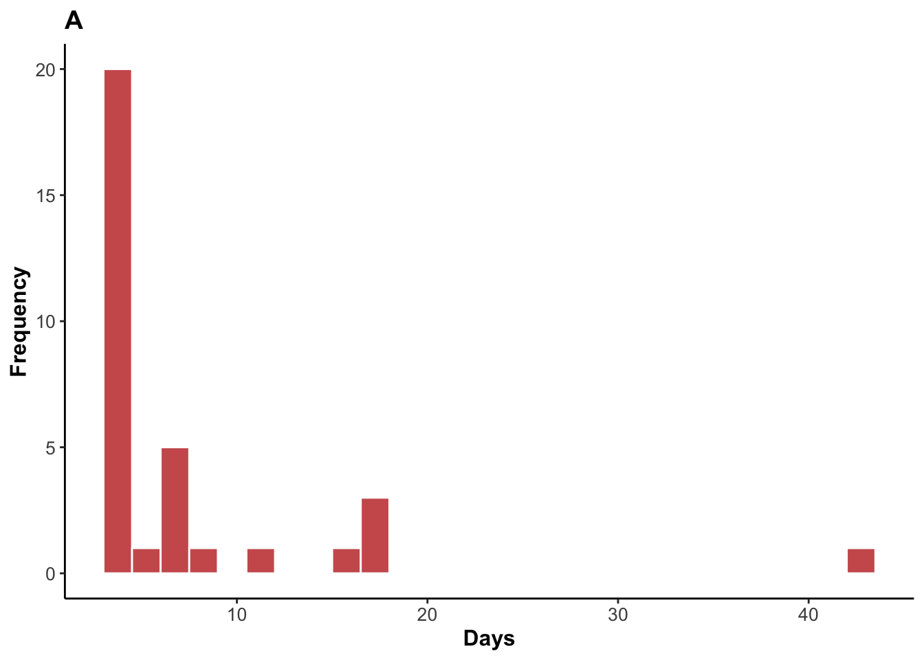
Histogram of skin clearance episodes.
ggplot(data = gas_skin_clearance, aes(x = time)) +
  geom_histogram(binwidth = 1, boundary = 0, fill = "indianred", color = "white") +
  labs(title = "B", x = "Days", y = "Frequency") +
  theme(plot.title = element_text(face = "bold", size = 14),
        axis.title = element_text(face = "bold", size = 12),
        axis.text = element_text(size = 10),
        panel.grid.major = element_blank(),
        panel.grid.minor = element_blank(),
        panel.background = element_blank(),
        panel.border = element_blank(),
        axis.line = element_line(size = 0.5, color = "black"),
        legend.position = "none")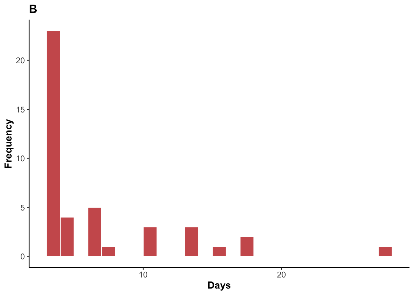
Median throat clearance time and range.
gas_throat_clearance |>
  reframe(median = median(time), range = range(time))
# A tibble: 2 × 2
median range
<dbl> <dbl>
1 4 3
2 4 42.5Median skin clearance time and range.
gas_skin_clearance |>
  reframe(median = median(time), range = range(time))
# A tibble: 2 × 2
median range
<dbl> <dbl>
1 4 3
2 4 27.5Wilcoxon Rank Sum of difference between throat and skin clearance time.
wilcox.test(gas_skin_clearance$time,gas_throat_clearance$time)Warning in wilcox.test.default(gas_skin_clearance$time,
gas_throat_clearance$time): cannot compute exact p-value with ties
    Wilcoxon rank sum test with continuity correction

data:  gas_skin_clearance$time and gas_throat_clearance$time
W = 728.5, p-value = 0.8442
alternative hypothesis: true location shift is not equal to 0
Antibiotic prescribing at the start of throat clearance episodes.
gas_throat_clearance |>
  filter(abx_start == 1) |>
  print(width = Inf)
# A tibble: 2 × 15
pid startdate enddate nextnegdate abx abx_start any_abx sx_start
<chr> <dbl> <dbl> <dbl> <dbl> <dbl> <dbl> <dbl>
1 10406C 19018 19018 19026 1 1 1 0
2 09506H 18997 18997 19005 1 1 1 0
sx_middle sx_end emm_type valid time gap any_sx
<dbl> <dbl> <chr> <chr> <dbl> <dbl> <dbl>
1 0 0 56 Yes 4 8 0
2 0 0 55 Yes 4 8 0Antibiotic prescribing at the end of throat clearance episodes.
gas_throat_clearance |>
  filter(abx == 1) |>
  print(width = Inf)
# A tibble: 3 × 15
pid startdate enddate nextnegdate abx abx_start any_abx sx_start
<chr> <dbl> <dbl> <dbl> <dbl> <dbl> <dbl> <dbl>
1 10406C 19018 19018 19026 1 1 1 0
2 08418C 19044 19059 19065 1 0 1 0
3 09506H 18997 18997 19005 1 1 1 0
sx_middle sx_end emm_type valid time gap any_sx
<dbl> <dbl> <chr> <chr> <dbl> <dbl> <dbl>
1 0 0 56 Yes 4 8 0
2 1 1 169.1 Yes 18 6 1
3 0 0 55 Yes 4 8 0Pyoderma symptoms at the start of skin clearance episodes.
gas_skin_clearance |>
  filter(sx_start == 1) |>
  print(width = Inf)
# A tibble: 7 × 15
pid startdate enddate nextnegdate abx abx_start any_abx sx_start
<chr> <dbl> <dbl> <dbl> <dbl> <dbl> <dbl> <dbl>
1 25522K 19194 19194 19201 1 1 1 1
2 11011B 19094 19094 19107 1 1 1 1
3 09304C 19215 19215 19221 1 1 1 1
4 29027H 19150 19165 19171 0 1 1 1
5 29028K 19185 19185 19193 1 1 1 1
6 05110F 19009 19009 19016 0 0 0 1
7 29504E 19009 19009 19019 1 1 1 1
sx_middle sx_end emm_type valid time gap any_sx
<dbl> <dbl> <chr> <chr> <dbl> <dbl> <dbl>
1 0 0 44 Yes 3.5 7 1
2 0 0 218.1 Yes 6.5 13 1
3 0 0 207 Yes 3 6 1
4 0 0 119.2 Yes 18 6 1
5 0 0 119.2 Yes 4 8 1
6 0 0 4.21 Yes 3.5 7 1
7 0 0 71 Yes 5 10 1Pyoderma symptoms and antibiotic prescribing at the start of skin clearance episodes.
gas_skin_clearance |>
  filter(sx_start == 1 & abx_start == 1) |>
  print(width = Inf)
# A tibble: 6 × 15
pid startdate enddate nextnegdate abx abx_start any_abx sx_start
<chr> <dbl> <dbl> <dbl> <dbl> <dbl> <dbl> <dbl>
1 25522K 19194 19194 19201 1 1 1 1
2 11011B 19094 19094 19107 1 1 1 1
3 09304C 19215 19215 19221 1 1 1 1
4 29027H 19150 19165 19171 0 1 1 1
5 29028K 19185 19185 19193 1 1 1 1
6 29504E 19009 19009 19019 1 1 1 1
sx_middle sx_end emm_type valid time gap any_sx
<dbl> <dbl> <chr> <chr> <dbl> <dbl> <dbl>
1 0 0 44 Yes 3.5 7 1
2 0 0 218.1 Yes 6.5 13 1
3 0 0 207 Yes 3 6 1
4 0 0 119.2 Yes 18 6 1
5 0 0 119.2 Yes 4 8 1
6 0 0 71 Yes 5 10 1Single visit skin clearance episodes with symptoms and antibiotics at the start.
gas_skin_clearance |>
  filter(sx_start == 1 & abx_start == 1 & startdate == enddate) |>
  print(width = Inf)
# A tibble: 5 × 15
pid startdate enddate nextnegdate abx abx_start any_abx sx_start
<chr> <dbl> <dbl> <dbl> <dbl> <dbl> <dbl> <dbl>
1 25522K 19194 19194 19201 1 1 1 1
2 11011B 19094 19094 19107 1 1 1 1
3 09304C 19215 19215 19221 1 1 1 1
4 29028K 19185 19185 19193 1 1 1 1
5 29504E 19009 19009 19019 1 1 1 1
sx_middle sx_end emm_type valid time gap any_sx
<dbl> <dbl> <chr> <chr> <dbl> <dbl> <dbl>
1 0 0 44 Yes 3.5 7 1
2 0 0 218.1 Yes 6.5 13 1
3 0 0 207 Yes 3 6 1
4 0 0 119.2 Yes 4 8 1
5 0 0 71 Yes 5 10 1Other symptoms (pharyngitis) and antibiotic prescribing at the start of skin clearance episodes.
# Other symptoms at start of episode
gas_skin_clearance |>
  filter(sx_start == 0 & abx_start == 1) |>
  print(width = Inf)
# A tibble: 1 × 15
pid startdate enddate nextnegdate abx abx_start any_abx sx_start
<chr> <dbl> <dbl> <dbl> <dbl> <dbl> <dbl> <dbl>
1 06106A 19124 19124 19138 1 1 1 0
sx_middle sx_end emm_type valid time gap any_sx
<dbl> <dbl> <chr> <chr> <dbl> <dbl> <dbl>
1 0 0 44 Yes 7 14 0Any antibiotic prescribing for skin clearance episodes.
gas_skin_clearance |>
  filter(any_abx == 1) |>
  print(width = Inf)
# A tibble: 10 × 15
pid startdate enddate nextnegdate abx abx_start any_abx sx_start
<chr> <dbl> <dbl> <dbl> <dbl> <dbl> <dbl> <dbl>
1 25520H 19005 19011 19027 1 0 1 0
2 25522K 19194 19194 19201 1 1 1 1
3 11011B 19094 19094 19107 1 1 1 1
4 06106A 19124 19124 19138 1 1 1 0
5 09304C 19215 19215 19221 1 1 1 1
6 29027H 19150 19165 19171 0 1 1 1
7 29028K 19185 19185 19193 1 1 1 1
8 29504E 19009 19009 19019 1 1 1 1
9 13508F 19124 19138 19142 1 0 1 0
10 08207K 19030 19037 19045 1 0 1 0
sx_middle sx_end emm_type valid time gap any_sx
<dbl> <dbl> <chr> <chr> <dbl> <dbl> <dbl>
1 1 1 55 Yes 14 16 1
2 0 0 44 Yes 3.5 7 1
3 0 0 218.1 Yes 6.5 13 1
4 0 0 44 Yes 7 14 0
5 0 0 207 Yes 3 6 1
6 0 0 119.2 Yes 18 6 1
7 0 0 119.2 Yes 4 8 1
8 0 0 71 Yes 5 10 1
9 1 1 65.7 Yes 16 4 1
10 1 1 171.1 Yes 11 8 1Any antibiotic prescribing for throat clearance episodes.
gas_throat_clearance |>
  filter(any_abx == 1) |>
  print(width = Inf)
# A tibble: 4 × 15
pid startdate enddate nextnegdate abx abx_start any_abx sx_start
<chr> <dbl> <dbl> <dbl> <dbl> <dbl> <dbl> <dbl>
1 10406C 19018 19018 19026 1 1 1 0
2 08418C 19044 19059 19065 1 0 1 0
3 09506H 18997 18997 19005 1 1 1 0
4 05206G 19012 19051 19058 0 0 1 0
sx_middle sx_end emm_type valid time gap any_sx
<dbl> <dbl> <chr> <chr> <dbl> <dbl> <dbl>
1 0 0 56 Yes 4 8 0
2 1 1 169.1 Yes 18 6 1
3 0 0 55 Yes 4 8 0
4 1 0 218.1 Yes 42.5 7 1Wilcox test for difference in antibiotic prescribing between throat and skin clearance episodes.
wilcox.test(gas_skin_clearance$any_abx,gas_throat_clearance$any_abx)Warning in wilcox.test.default(gas_skin_clearance$any_abx,
gas_throat_clearance$any_abx): cannot compute exact p-value with ties
    Wilcoxon rank sum test with continuity correction

data:  gas_skin_clearance$any_abx and gas_throat_clearance$any_abx
W = 788.5, p-value = 0.2205
alternative hypothesis: true location shift is not equal to 0
Wilcox test for antibiotic use impact on throat clearance episode length.
gas_throat_clearance %>%
  group_by(any_abx) %>%
  summarise(nrow = table(any_abx),
            median = median(time))
# A tibble: 2 × 3
any_abx nrow median
<dbl> <table[1d]> <dbl>
1 0 29 4
2 1 4 11wilcox.test(time ~ any_abx, data = gas_throat_clearance)Warning in wilcox.test.default(x = DATA[[1L]], y = DATA[[2L]], ...): cannot
compute exact p-value with ties
    Wilcoxon rank sum test with continuity correction

data:  time by any_abx
W = 31.5, p-value = 0.1457
alternative hypothesis: true location shift is not equal to 0
Wilcox test for antibiotic use impact on skin clearance episode length.
gas_skin_clearance |>
  group_by(any_abx) |>
  summarise(nrow = table(any_abx),
            median = median(time))
# A tibble: 2 × 3
any_abx nrow median
<dbl> <table[1d]> <dbl>
1 0 33 4
2 1 10 6.75wilcox.test(time ~ any_abx, data = gas_skin_clearance)Warning in wilcox.test.default(x = DATA[[1L]], y = DATA[[2L]], ...): cannot
compute exact p-value with ties
    Wilcoxon rank sum test with continuity correction

data:  time by any_abx
W = 112.5, p-value = 0.1301
alternative hypothesis: true location shift is not equal to 0
Demographic risk factors for carriage and infection
The events_long dataframe is a long dataframe set up using tmerge to allow for survival (time-to-event) analysis for each of the relevant events. For each participant, the time period between each visit is a row of the dataframe with a start time (tstart) and stop time (tstop). gap indicates whether the period was a gap in follow up or not (these will be filtered out before the analysis. The events (gas_pharyngitis, gas_throat_carriage, gas_pyoderma and gas_skin_carriage) are coded as “events” whereby for example if an event occurred at timepoint 65, the event will be positive (1) for the row where tstop is 65. Rainy season (rain) and household size (hhsize) are coded as time-varying covariates whereby they change over time for each participants. Age group (age_grp) and sex (sex) are constant covariates that do not change. Household ID number is represented by hid while pid is the participant ID number.
load("./Data/events_long.RData")

head(events_long)
pid age_grp sex hid tstart tstop gap gas_pharyngitis gas_pyoderma
1 00201K Over 18 years Male 2 0 43 0 0 0
2 00201K Over 18 years Male 2 43 57 0 0 0
3 00201K Over 18 years Male 2 57 71 1 0 0
4 00201K Over 18 years Male 2 71 93 1 0 0
5 00201K Over 18 years Male 2 93 120 1 0 0
6 00201K Over 18 years Male 2 120 161 1 0 0
gas_throat_carriage gas_skin_carriage hhsize rain
1 0 0 5 1
2 0 0 5 1
3 0 0 5 1
4 0 0 6 0
5 0 0 6 0
6 0 0 6 0Using the coxph command in the survival package, we can perform Andersen-Gill regression, which is as extension of the Cox Proportional Hazards regression model which allows for recurrent events (assuming independence between events) by including pid in the model, accounts for household clustering by including hid in the model and uses robust standard errors. Age group, sex, household size and season are all added to the multivariable model for each event.
First we filter out gaps in follow up, then we write a function to perform the analysis.
events_long <- events_long |>
  filter(gap == 0) |>
  select(!gap)

coxag <- function(outcome,data) {

  outcome <- substitute(outcome)

  model <- coxph(Surv(tstart, tstop, eval(outcome, data)) ~ rain + sex + age_grp + hhsize, cluster = hid, id = pid, data = data)
  tb <- model |>
    tbl_regression(exponentiate = TRUE,
                   label = list(rain ~ "Rainy season", age_grp ~ "Age Group", sex ~ "Sex", hhsize ~ "Household size")) |>
    add_nevent() |>
    add_global_p() |>
    bold_labels() |>
    bold_p(t = 0.05) |>
    modify_header(list(label ~ "**Characteristic**"))
  tb

}
Then run the function for each event.
Pharyngeal carriage.
coxag(gas_throat_carriage, events_long)Warning in Anova.coxph(mod = x, type = type, ...): LR tests unavailable with robust variances
Wald tests substitutedWarning in printHypothesis(L, rhs, names(b)): one or more coefficients in the hypothesis include
arithmetic operators in their names;
the printed representation of the hypothesis will be omitted| Characteristic | Event N | HR1 | 95% CI1 | p-value |
|---|---|---|---|---|
| Rainy season | 37 | 5.67 | 2.19, 14.7 | <0.001 |
| Sex | 37 | 0.2 | ||
| Male | — | — | ||
| Female | 0.71 | 0.40, 1.26 | ||
| Age Group | 37 | <0.001 | ||
| Over 18 years | — | — | ||
| 0-5 years | 2.92 | 1.53, 5.58 | ||
| 5-12 years | 4.80 | 1.71, 13.5 | ||
| 12-18 years | 0.91 | 0.18, 4.64 | ||
| Household size | 37 | 1.03 | 1.00, 1.05 | 0.030 |
| 1 HR = Hazard Ratio, CI = Confidence Interval | ||||
Skin carriage.
coxag(gas_skin_carriage, events_long)Warning in Anova.coxph(mod = x, type = type, ...): LR tests unavailable with robust variances
Wald tests substitutedWarning in printHypothesis(L, rhs, names(b)): one or more coefficients in the hypothesis include
arithmetic operators in their names;
the printed representation of the hypothesis will be omitted| Characteristic | Event N | HR1 | 95% CI1 | p-value |
|---|---|---|---|---|
| Rainy season | 38 | 0.42 | 0.09, 1.91 | 0.3 |
| Sex | 38 | 0.030 | ||
| Male | — | — | ||
| Female | 0.45 | 0.22, 0.92 | ||
| Age Group | 38 | 0.022 | ||
| Over 18 years | — | — | ||
| 0-5 years | 22.7 | 3.08, 167 | ||
| 5-12 years | 18.4 | 2.70, 126 | ||
| 12-18 years | 16.5 | 2.58, 106 | ||
| Household size | 38 | 1.00 | 0.98, 1.01 | 0.7 |
| 1 HR = Hazard Ratio, CI = Confidence Interval | ||||
Pharyngitis.
coxag(gas_pharyngitis, events_long)Warning in Anova.coxph(mod = x, type = type, ...): LR tests unavailable with robust variances
Wald tests substitutedWarning in printHypothesis(L, rhs, names(b)): one or more coefficients in the hypothesis include
arithmetic operators in their names;
the printed representation of the hypothesis will be omitted| Characteristic | Event N | HR1 | 95% CI1 | p-value |
|---|---|---|---|---|
| Rainy season | 16 | 3.00 | 1.10, 8.22 | 0.032 |
| Sex | 16 | 0.5 | ||
| Male | — | — | ||
| Female | 0.75 | 0.31, 1.77 | ||
| Age Group | 16 | 0.055 | ||
| Over 18 years | — | — | ||
| 0-5 years | 0.43 | 0.11, 1.69 | ||
| 5-12 years | 2.86 | 0.95, 8.58 | ||
| 12-18 years | 1.15 | 0.38, 3.43 | ||
| Household size | 16 | 1.04 | 1.02, 1.07 | <0.001 |
| 1 HR = Hazard Ratio, CI = Confidence Interval | ||||
Pyoderma.
coxag(gas_pyoderma, events_long)Warning in Anova.coxph(mod = x, type = type, ...): LR tests unavailable with robust variances
Wald tests substitutedWarning in printHypothesis(L, rhs, names(b)): one or more coefficients in the hypothesis include
arithmetic operators in their names;
the printed representation of the hypothesis will be omitted| Characteristic | Event N | HR1 | 95% CI1 | p-value |
|---|---|---|---|---|
| Rainy season | 82 | 1.14 | 0.34, 3.84 | 0.8 |
| Sex | 82 | <0.001 | ||
| Male | — | — | ||
| Female | 0.34 | 0.19, 0.61 | ||
| Age Group | 82 | <0.001 | ||
| Over 18 years | — | — | ||
| 0-5 years | 7.00 | 2.78, 17.6 | ||
| 5-12 years | 6.60 | 2.77, 15.7 | ||
| 12-18 years | 2.69 | 1.18, 6.12 | ||
| Household size | 82 | 1.01 | 1.00, 1.03 | 0.14 |
| 1 HR = Hazard Ratio, CI = Confidence Interval | ||||
Emm-type diversity
The dataframe emm_types contains emm-typing data from all of the available isolates.
load("./Data/emm_types.RData")

head(emm_types)
pid date sample_type mrc_species isolate_id brussels_species
1 14704G 2022-01-18 ops 2 00318PG2 2
2 25521A 2022-01-19 ops 2 00395PG2 2
3 14006F 2022-01-20 ops 2 00286PG2 2
4 29008B 2022-01-25 ops 2 00408PG2 2
5 08414K 2022-01-24 ops 2 00152PC2 2
6 29028K 2021-11-29 ops 2 00467PG2 2
emm_type no_growth species_change small_colony new_subtype
1 stc1400.0 0 0 0 0
2 emm31.11 0 0 0 1
3 stg354.3 0 0 0 1
4 stg480.6 0 0 0 0
5 stg211.0 0 0 0 0
6 stg480.6 0 0 0 0Number of StrepA isolates successfully regrown and sent to MBLB.
emm_types |>
  filter(mrc_species == 1) |>
  nrow()
[1] 227Number of isolates with no growth at MBLB.
emm_types |>
  filter(mrc_species == 1 & no_growth == 1) |>
  nrow()
[1] 1Number of isolates latex tested as non-Group A Streptococcus at MBLB.
emm_types |>
  filter(mrc_species == 1 & species_change == 1) |>
  nrow()
[1] 6Number of StrepA isolates successfully emm-typed.
emm_types |>
  filter(brussels_species == 1) |>
  nrow()
[1] 221Number of unique emm-types.
emm_types |>
  filter(brussels_species == 1) |>
  distinct(emm_type) |>
  nrow()
[1] 57Number of new emm sub-types.
emm_types |>
  filter(brussels_species == 1 & new_subtype == 1) |>
  nrow()
[1] 3The dataframe event_list contains details with emm-type of each StrepA event identified.
load("./Data/event_list.RData")

head(event_list)
# A tibble: 6 × 6
pid date visit emm_type type hid
<chr> <date> <chr> <chr> <chr> <chr>
1 01603C 2022-08-01 mv11 emm88.11 pharyngitis 016
2 02106J 2021-12-16 mv4 emm113.0 pharyngitis 021
3 04011K 2021-07-29 mv0 nt pharyngitis 040
4 05903H 2022-03-01 mv7 emm55.0 pharyngitis 059
5 07904H 2021-11-08 uv emm183.2 pharyngitis 079
6 08418C 2022-03-08 wv emm169.1 pharyngitis 084 Number of events with emm-typed isolate.
event_list |>
  filter(emm_type != "nt") |>
  nrow()
[1] 179Household secondary attack rate
The dataframe between_visit_linked_events contains data on how many people were swabbed from the same household within 3-42 days after a StrepA event, and how many were of the same emm-type.
load("./Data/between_visit_linked_events.RData")

head(between_visit_linked_events)
pid date visit emm_type type hid total_swabs
1 01603C 2022-08-01 mv11 emm88.11 pharyngitis 016 6
2 02106J 2021-12-16 mv4 emm113.0 pharyngitis 021 6
3 05903H 2022-03-01 mv7 emm55.0 pharyngitis 059 13
4 07904H 2021-11-08 uv emm183.2 pharyngitis 079 27
5 08418C 2022-03-08 wv emm169.1 pharyngitis 084 43
6 13512H 2021-10-20 uv emm65.4 pharyngitis 135 27
total_people_swabbed total_sec_pos total_sec_pos_emm
1 3 0 0
2 3 0 0
3 6 0 0
4 8 1 0
5 19 2 0
6 9 0 0Total number of “index” events - events where someone in the household was swabbed 3-42 days later.
between_visit_linked_events |>
  nrow()
[1] 169Total number of “index” events by event type.
between_visit_linked_events |>
  group_by(type) |>
  summarise(n = n())
# A tibble: 4 × 2
type n
<chr> <int>
1 pharyngitis 15
2 pyoderma 81
3 skin_carriage 33
4 throat_carriage 40Total number of “epidemiologically linked” (not necessarily of the same emm-type) secondary events that occurred.
between_visit_linked_events |>
  summarise(x = sum(total_sec_pos))
x
1 128Total number of “epidemiologically linked” secondary events by index event type.
between_visit_linked_events |>
  group_by(type) |>
  summarise(x = sum(total_sec_pos))
# A tibble: 4 × 2
type x
<chr> <dbl>
1 pharyngitis 19
2 pyoderma 59
3 skin_carriage 20
4 throat_carriage 30Total number of “emm-type linked” (of the same emm-type) secondary events that occurred.
between_visit_linked_events |>
  summarise(x = sum(total_sec_pos_emm))
x
1 18Total number of “emm-type linked” secondary events by index event type.
between_visit_linked_events |>
  group_by(type) |>
  summarise(x = sum(total_sec_pos_emm))
# A tibble: 4 × 2
type x
<chr> <dbl>
1 pharyngitis 3
2 pyoderma 11
3 skin_carriage 2
4 throat_carriage 2Mean household secondary attack rate (HSAR) with confidence intervals for epidemiologically linked and emm-type linked events.
between_visit_linked_events |>
  mutate(sar = total_sec_pos / total_people_swabbed * 100,
         sar_emm = total_sec_pos_emm / total_people_swabbed * 100) |>
  summarise(mean_sar = mean(sar),
            mean_sar_emm = mean(sar_emm),
            n = n(),
            sd1 = sd(sar),
            sd2 = sd(sar_emm)) |>
  mutate(
    se1 = sd1 / sqrt(n),
    lower_ci1 = mean_sar - qt(0.975, df = n - 1) * se1,
    upper_ci1 = mean_sar + qt(0.975, df = n - 1) * se1,
    se2 = sd2 / sqrt(n),
    lower_ci2 = mean_sar_emm - qt(0.975, df = n - 1) * se2,
    upper_ci2 = mean_sar_emm + qt(0.975, df = n - 1) * se2)
mean_sar mean_sar_emm n sd1 sd2 se1 lower_ci1 upper_ci1
1 4.887861 0.7393453 169 9.201307 3.066412 0.7077928 3.490547 6.285175
se2 lower_ci2 upper_ci2
1 0.2358779 0.2736787 1.205012Mean household secondary attack rate (HSAR) with confidence intervals for epidemiologically linked and emm-type linked events by index event type.
between_visit_linked_events |>
  group_by(type) |>
  mutate(sar = total_sec_pos / total_people_swabbed * 100,
         sar_emm = total_sec_pos_emm / total_people_swabbed * 100) |>
  summarise(mean_sar = mean(sar),
            mean_sar_emm = mean(sar_emm),
            n = n(),
            sd1 = sd(sar),
            sd2 = sd(sar_emm)) |>
  mutate(
    se1 = sd1 / sqrt(n),
    lower_ci1 = mean_sar - qt(0.975, df = n - 1) * se1,
    upper_ci1 = mean_sar + qt(0.975, df = n - 1) * se1,
    se2 = sd2 / sqrt(n),
    lower_ci2 = mean_sar_emm - qt(0.975, df = n - 1) * se2,
    upper_ci2 = mean_sar_emm + qt(0.975, df = n - 1) * se2) |>
  print(width = Inf)
# A tibble: 4 × 12
type mean_sar mean_sar_emm n sd1 sd2 se1 lower_ci1
<chr> <dbl> <dbl> <int> <dbl> <dbl> <dbl> <dbl>
1 pharyngitis 6.76 0.797 15 11.1 2.17 2.86 0.625
2 pyoderma 4.24 0.807 81 8.18 3.37 0.909 2.43
3 skin_carriage 5.96 0.577 33 9.95 2.60 1.73 2.43
4 throat_carriage 4.62 0.714 40 9.94 3.15 1.57 1.44
upper_ci1 se2 lower_ci2 upper_ci2
<dbl> <dbl> <dbl> <dbl>
1 12.9 0.561 -0.406 2.00
2 6.04 0.375 0.0618 1.55
3 9.48 0.452 -0.344 1.50
4 7.81 0.499 -0.294 1.72Household transmission of emm-types
The within_visit_linkages dataframe contains details of all linkages that occurred of identical emm-type within a 0-2 day period - where directionality is not possible to determine.
load(file = "./Data/within_visit_linkages.RData")

head(within_visit_linkages)
# A tibble: 6 × 8
source_pid source_date source_event_type recipient_pid recipient_date
<chr> <date> <chr> <chr> <date>
1 00204D 2022-01-24 pyoderma 00205G 2022-01-24
2 00205G 2022-01-24 pyoderma 00204D 2022-01-24
3 06207J 2022-04-27 pyoderma 06206E 2022-04-27
4 08306E 2021-09-15 pyoderma 08308G 2021-09-15
5 08416D 2021-09-20 pyoderma 08434D 2021-09-20
6 10406C 2022-01-26 pyoderma 10407A 2022-01-26
# ℹ 3 more variables: recipient_event_type <chr>, emm_type <chr>, lag <int>The between_visit_linkages dataframe contains details of all linkages that occurred of identical emm-type within a 3-42 day period - where directionality is known.
load(file = "./Data/between_visit_linkages.RData")

head(between_visit_linkages)
# A tibble: 6 × 8
source_pid source_date source_event_type recipient_pid recipient_date
<chr> <date> <chr> <chr> <date>
1 29018E 2021-11-02 pharyngitis 29030E 2021-11-16
2 08433F 2021-09-30 pharyngitis 08402B 2021-10-18
3 08433F 2021-09-30 pharyngitis 08430J 2021-10-18
4 08416D 2021-09-20 pyoderma 08433F 2021-09-30
5 08416D 2021-09-20 pyoderma 08402B 2021-10-18
6 08416D 2021-09-20 pyoderma 08430J 2021-10-18
# ℹ 3 more variables: recipient_event_type <chr>, emm_type <chr>, lag <int>Number of within-visit linkages.
within_visit_linkages |>
  nrow()
[1] 42Number of between-visit linkages.
between_visit_linkages |>
  nrow()
[1] 18Within-visit linkages by source and recipient event type (though directionality unknown).
within_visit_linkages |>
  tbl_cross(
    col = source_event_type,
row = recipient_event_type, percent = "cell")| source_event_type | Total | |||
|---|---|---|---|---|
| pyoderma | skin_carriage | throat_carriage | ||
| recipient_event_type | ||||
| pyoderma | 8 (19%) | 5 (12%) | 1 (2.4%) | 14 (33%) |
| skin_carriage | 5 (12%) | 12 (29%) | 3 (7.1%) | 20 (48%) |
| throat_carriage | 1 (2.4%) | 3 (7.1%) | 4 (9.5%) | 8 (19%) |
| Total | 14 (33%) | 20 (48%) | 8 (19%) | 42 (100%) |
Between-visit linkages by source and recipient event type.
between_visit_linkages |>
  tbl_cross(
    col = source_event_type,
row = recipient_event_type, percent = "cell")| source_event_type | Total | ||||
|---|---|---|---|---|---|
| pharyngitis | pyoderma | skin_carriage | throat_carriage | ||
| recipient_event_type | |||||
| pharyngitis | 0 (0%) | 3 (17%) | 0 (0%) | 0 (0%) | 3 (17%) |
| pyoderma | 0 (0%) | 3 (17%) | 2 (11%) | 2 (11%) | 7 (39%) |
| skin_carriage | 1 (5.6%) | 3 (17%) | 0 (0%) | 0 (0%) | 4 (22%) |
| throat_carriage | 2 (11%) | 2 (11%) | 0 (0%) | 0 (0%) | 4 (22%) |
| Total | 3 (17%) | 11 (61%) | 2 (11%) | 2 (11%) | 18 (100%) |
Median serial interval for between visit linkages.
between_visit_linkages |>
  summarise(median = median(lag))
# A tibble: 1 × 1
median
<dbl>
1 28Median serial interval by source event.
between_visit_linkages |>
  group_by(source_event_type) |>
  summarise(med = median(lag))
# A tibble: 4 × 2
source_event_type med
<chr> <dbl>
1 pharyngitis 18
2 pyoderma 28
3 skin_carriage 24.5
4 throat_carriage 18 The dataframes within_visit_translocations and between_visit_translocations contain details of occasions where a change of event type occurred in one individiaul within the defined transmission windows.
load(file = "./Data/within_visit_translocations.RData")

load(file = "./Data/between_visit_translocations.RData")

head(within_visit_translocations)
# A tibble: 5 × 8
source_pid source_date source_event_type recipient_pid recipient_date
<chr> <date> <chr> <chr> <date>
1 05110F 2022-01-17 pyoderma 05110F 2022-01-17
2 10406C 2022-01-26 pyoderma 10406C 2022-01-26
3 11011B 2022-04-12 pyoderma 11011B 2022-04-12
4 25522K 2022-07-21 pyoderma 25522K 2022-07-21
5 29504E 2022-01-17 pyoderma 29504E 2022-01-17
# ℹ 3 more variables: recipient_event_type <chr>, emm_type <chr>, lag <int>head(between_visit_translocations)# A tibble: 3 × 8
source_pid source_date source_event_type recipient_pid recipient_date
<chr> <date> <chr> <chr> <date>
1 29022J 2021-12-08 pyoderma 29022J 2021-12-13
2 25520H 2022-01-13 skin_carriage 25520H 2022-01-19
3 08207K 2022-02-07 skin_carriage 08207K 2022-02-14
# ℹ 3 more variables: recipient_event_type <chr>, emm_type <chr>, lag <int>Number of within-visit translocations.
within_visit_translocations |>
  nrow()
[1] 5Number of between-visit translocations.
between_visit_translocations |>
  nrow()
[1] 3Within-visit translocation source/recipient sites.
within_visit_translocations |>
  tbl_cross(
    col = source_event_type,
row = recipient_event_type, percent = "cell")| source_event_type | Total | |
|---|---|---|
| pyoderma | ||
| recipient_event_type | ||
| skin_carriage | 4 (80%) | 4 (80%) |
| throat_carriage | 1 (20%) | 1 (20%) |
| Total | 5 (100%) | 5 (100%) |
Between-visit translocation source/recipient sites.
between_visit_translocations |>
  tbl_cross(
    col = source_event_type,
row = recipient_event_type, percent = "cell")| source_event_type | Total | ||
|---|---|---|---|
| pyoderma | skin_carriage | ||
| recipient_event_type | |||
| pyoderma | 0 (0%) | 2 (67%) | 2 (67%) |
| throat_carriage | 1 (33%) | 0 (0%) | 1 (33%) |
| Total | 1 (33%) | 2 (67%) | 3 (100%) |